total_bill | tip | percent_tip | smoker | day | time | size |
|---|---|---|---|---|---|---|
17.59 | 2.64 | 0.1500853 | No | Sat | Dinner | 3 |
25.21 | 4.29 | 0.1701706 | Yes | Sat | Dinner | 2 |
31.27 | 5.00 | 0.1598977 | No | Sat | Dinner | 3 |
20.08 | 3.15 | 0.1568725 | No | Sat | Dinner | 3 |
16.00 | 2.00 | 0.1250000 | Yes | Thur | Lunch | 2 |
12 Review
Measuring the evidence for an alternate hypothesis
You never really understand a person until you consider things from his point of view. Until you climb inside of his skin and walk around in it.”
― Atticus Finch in “To Kill a Mockingbird” by Harper Lee
We will continue to study the data collected by a restaurant waiter in 1995, regarding bills and tips at lunch and dinner. A few rows of the dataset are shown below, for reference:
Thus far, we have focused on the null hypothesis, and how to make an argument for whether it is reasonable to believe or not.
But if we do find data that is inconsistent with the null - that is, if we reject the null hypothesis - what should we believe instead?
Recall from last chapter that we asked the research question:
Do people tend to spend more on their meal at Dinner than at Lunch?
This led us to define our null hypothesis as
H_0: \mu_D = \mu_L
Notice that in our research question, we began with the inherent expectation that dinners are more expensive than lunches. We have decided not to investigate the possibility that lunch costs more than dinner; we only want to determine if there is sufficient evidence to conclude dinner costs more than lunch, or if there is no evidence of a difference.
We have therefore not only made a decision here about what null hypothesis we are hoping to argue against. We have also narrowed down the possible truths that we plan to argue for; namely, that dinner costs more than lunch.
12.1 The Alternate Hypothesis
In the above example, our research question implied a particular alternate hypothesis a claim we are making that we hope the data will support. We might state our alternate hypothesis, (H_a), as:
H_a: \text{The true mean bill at dinner is higher than the true mean bill at lunch.}
or,
H_a: \mu_D > \mu_L
or
H_a: \mu_D - \mu_L > 0
All three of these are acceptable ways to state the an alternate hypothesis. It is also important that our null and alternate hypotheses are determined before we start analyzing the data. That is, we chose to research “dinner is more expensive than lunch” because we had that belief from previous experience, not because we had already seen that trend in our data.
Remember that all hypotheses, null or alternate, are making claims about parameters - in this case, the true means \mu_L and \mu_D.
In the last chapter, we found the sample mean bill price of lunch and dinner to be \bar{x}_L = \$16.23 and \bar{x}_D = \$21.15. There is no need for us to hypothesize about these summary statistics, since we know exactly what they are equal to! However, these statistics by themselves don’t tell us that the alternate hypothesis is definitely true - we could possibly have gotten different numbers if we’d studied a different week at the restaurant.
To fully address our research question, we found that the sample mean difference, \bar{x}_D - \bar{x}_L = \$4.97, was 2.47 standard deviations above zero. With our “magic simulation” of data from the null universe, we decided that this would only happen by chance 1.8% of the time. We there concluded that indeed, people spend more at dinners than at lunches.
In the end, we chose to reject the null hypothesis and accept the alternate hypothesis.
12.1.1 Direction of the alternate
What if, instead, we had asked the question:
Do people tend to spend more at Lunch than at Dinner?
In this version of the question, we begin with the assumption that lunch will have higher bills than dinner. Of course, the data does not support this assumption - but because we make our hypotheses before observing our data, this is a completely reasonable research question to study.
Our null hypothesis is still the idea that “nothing interesting is happening here” or “there is no relationship between the variables”. If lunch is more expensive than dinner, that is a relationship between Time and Total Bill. If dinner is more expensive than lunch - even though we are not studying that possibility - that still represents a relationship between Time and Total Bill.
Thus, our null hypothesis remains the same:
H_0: \mu_D = \mu_L
However, in this version of the analysis, we have a very different alternate hypothesis: that dinner bills are on average less than lunch bills.
H_a: \mu_D < \mu_L
When we analyze the data, the math is unchanged. We still find that
\bar{x}_D - \bar{x}_L = \$4.92
and we still find that this is 2.47 standard deviations above zero.
But now we must ask ourselves: what summary statistic would give us evidence for the alternate hypothesis? If \bar{x}_D - \bar{x}_L is a positive number, that tells us that dinners are more expensive; we wanted to show that dinner was less expensive. If the z-score is positive, that tells us that our observed difference of means was above zero; we wanted to show that it was below zero.
In other words, even though the z-score was large, we haven’t found evidence for our alternate hypothesis at all!
If we want to think about the p-value in this version of the analysis, we once again ask,
If we lived in a world where null hypothesis is true, how often would we see a statistic as extreme as the one from our data?
However, our definition of “extreme” has changed: we now consider “extremely high evidence” to be values where the mean bill at lunch is less than the mean bill at dinner, i.e., negative differences.
Let’s revisit our imaginary sample mean differences generated from the null universe:
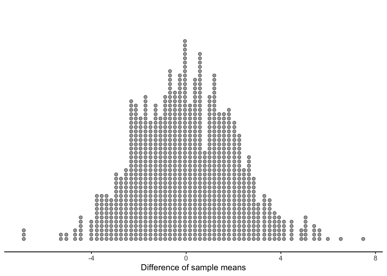
How often did our simulated data result in a difference of means that would be more evidence for the alternate hypothesis than what we saw in the data? Well, what we saw in the data was that dinners were $2.47 more. If we had seen that dinners were $2.00 more, that would still not be good news for our alternate hypothesis, but it would at least be better than $2.47. If we saw that the sample means were the same - a difference of $0 - that would be very consistent with the null hypothesis… but it would still be a “better” outcome for our alternate hypothesis than $4.92.
All this is to say that everything in the red area, to the left of the line we drew at $4.92, represents times when our simulated data resulted in more extreme values of the difference of sample means.
Since we said the blue area to the right of the cutoff was 1.8% (18 out of 1000) of the simulated values, we know that the red area is 98.2% of the simulated values.
So, what did we learn? We learned that in a world where the null hypothesis is true, we would get (by luck) better evidence for our alternate hypothesis 98.2% of the time!
We conclude, of course, that we found absolutely no evidence in favor of our alternate hypothesis. We fail to reject the null hypothesis, because our alternative was even more implausible.
12.1.2 Two-sided Hypotheses
What if we decide to be a bit more neutral in our study, and to not begin with any kind of assumptions about whether lunch or dinner is more expensive. We might ask,
Do people tend to spend different amounts of money at Dinner than at Lunch?
In this version, our alternate hypothesis is two-sided: we are interested in showing that dinner is more expensive or that lunch is more expensive. We would write this as
H_a: \mu_D \neq \mu_L
where the \neq symbol means “is not equal to”.
Our calculation of the summary statistic ($4.92) and z-score (2.47) is, of course, unchanged. But once again, we must rethink what it means to be “extreme” in the simulated statistics.
Certainly, as in our very first version of this analysis, any simulated differences of means over 4.92 would provide more evidence that \mu_D \> \mu_L. Now, though, we are also interested in evidence that \mu_L > \mu_D. What if we saw lunches be $4.92 more expensive than dinners, for a z-score of -2.47? That would be an equal amount of evidence for the alternate hypothesis; just in the other direction.
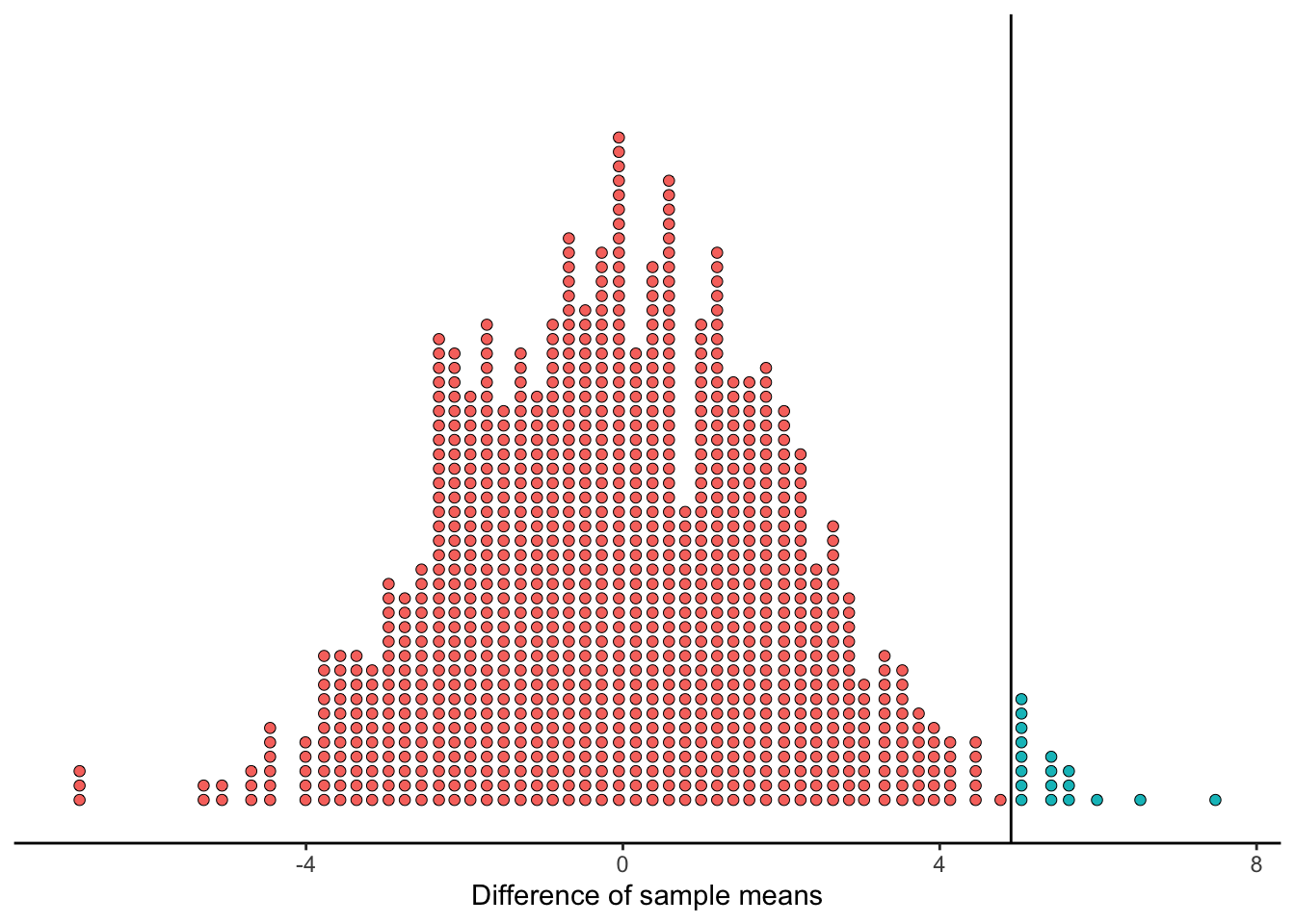
Thus, if our alternate hypothesis is two-sided, we have to count how often data from the null universe would be as extreme in either direction:
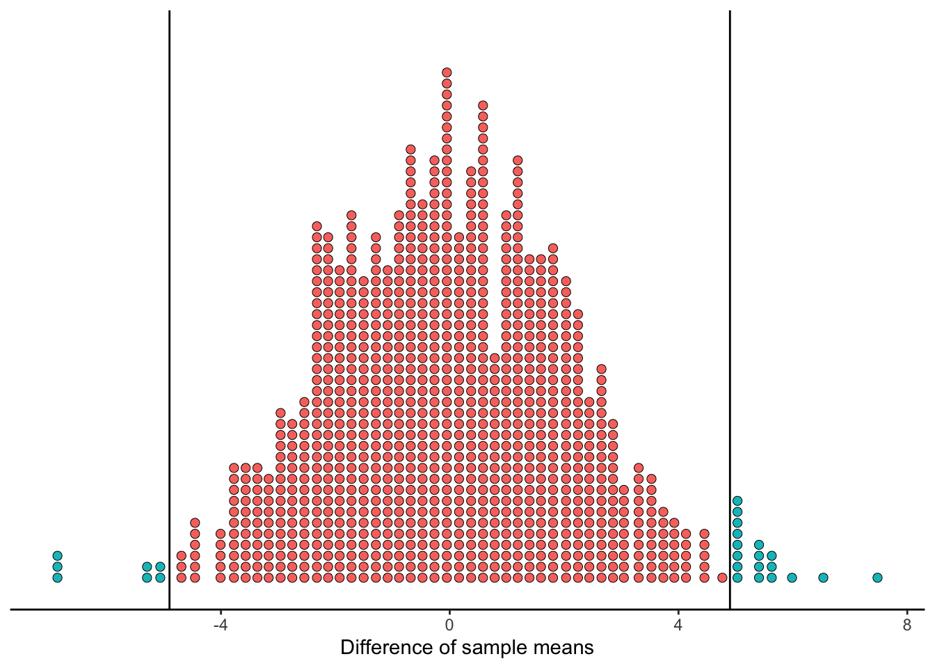
This time, we still have 18 simulated values above 4.92, and we also have 7 simulated values below -4.92.
Therefore, our p-value in this two-sided case is 25/1000 = 2.5%.
Since the p-value is still quite small, we would probably conclude that it’s not reasonable to assume our data came from a world where the null hypothesis is true. We reject the null hypothesis in favor of the alternate hypothesis: the true mean bill of lunch and dinner are not equal.
But we aren’t quite done. Imagine that the waiter returns to his manager and says, “Guess what! I’ve found evidence that people spend different amounts at lunch and dinner!” Of course, the manager’s first question is going to be, “Okay, but at which meal do they spend more?”
Our hypothesis was two-sided, and we had keep that in mind to quantify our evidence with a p-value. However, our conclusion still needs to make sense in the real world. In this case, we found evidence that people spend more at dinner than at lunch, on average.
12.2 Statistical significance
A question you might be asking yourself is, what counts as a “small enough” p-value?
If you observe data that could only happen 1% of the time if the null hypothesis were true, you probably feel pretty good about rejecting the null hypothesis. But what if your calculated statistic would have a 5% chance of occurring in a null universe? Or a 10% chance? 20%? At what point do you feel comfortable declaring that the null is probably not true?
There is no single correct answer to this question. It is up to the scientist to decide, in their specific scientific setting, how much evidence is sufficient to act on.
12.2.1 What’s in a name?
Statisticians use the word significant to refer to a p-value that is below the established threshold in a particular context.
This word can be very misleading, because in ordinary English, the word “significant” means “sufficiently great or important to be worthy of attention”. Before this chapter, you might have said that $5 is not a significant amount of money.
However, in the field of statistics, the word “significant” actually comes from the French word significant, which means “signifying” or “indicating”. Something is significant if it signifies a truth, not if it is large or impressive.
To a statistician or data scientist, saying “There was a mean difference of $4.92” is not interesting, because it does not give any information about uncertainty. Does the difference of around $5 signify that there is a true difference in average bills? We don’t know until we do the analysis that takes variability into account, and find a p-value.
Scientists will sometimes use the term statistical significance, to make it clear that they are referring to whether the data is signifying that the alternate hypothesis is true. In this book, we will usually use “significant” by itself; from now on, we always mean this in the statistical sense!
12.2.2 Low significance thresholds
There are plenty of times when the analysis you are performing is exploratory. You have gathered a dataset with the goal of uncovering some interesting trends, or finding some ideas for future analysis. The study is not being done to “prove” some main hypothesis, but rather, to get a broad picture of the data landscape. In these situations, you might be satisfied with a relatively high p-value.
For example, suppose you are studying whether certain fertilizers negatively impact an ecosystem. It is very expensive and time-consuming to apply fertilizers to many samples of garden sections and then analyze the bacteria life in the soils. Instead, you might perform a preliminary version of the experiment, with a smaller sample size.
Then, when you collect the data, you note that Fertilizer A did not significantly lower bacteria growth (p-value of 0.4), but Fertilizer B may have lowered bacteria growth (p-value of 0.12).
You aren’t ready to run through the halls of Home Depot shouting “Don’t buy Fertilizer B!” After all, there is a 12% chance that your observed lower bacteria growth could happen with no impact from the fertilizer.
But you did find enough evidence to suggest a future study. You can now re-do your experiment, with a much larger sample size, and you don’t need to waste your resources including Fertilizer A.
Moderate p-values are not sufficient to suggest major changes in policy or procedure, but they might suggest, “Here is something worth investigating further.”
12.2.3 High significance thresholds
On the other hand, some scientific studies require a very high level of certainty to make a conclusion.
One such example is the area of theoretical physics. In 2012, researchers at CERN laboratories in Switzerland discovered a particle called the Higgs boson. But what does it mean to “discover” a particle, when the existence of that partical had been theorized mathematically since 1964? The process of “proving” the particle’s existence consisted of a series of complicated experiments, in which subatomic particles are forced to crash together at high speeds, and properties of the explosion are measured.
Although this experiment feels very precise and controlled, it is still a scenario where data is being collected and small random changes to the environment lead to sampling variability. Therefore, researchers needed to decide how much evidence they would accept in order to declare the particle “discovered”.
In the 2012 experiments, they chose a cutoff of 0.0000003. That is, only a p-value of less than 0.00003% would be considered significant.
Any time a study is being performed where the conclusion will have a major impact - such as changing the basic understanding of physics theory, releasing a new medication into a population, or making a multi-million-dollar business decision - it is important to have strong evidence.
12.2.4 The 0.05 threshold
In principle, the p-value cutoff for significance should be a decision made by the scientist, based on the context of the study.
In practice, unfortunately, not everyone follows ethical scientific behavior.
Imagine that you have worked for many years to perform an experiment. You had set your significance threshold as 0.02, because you think that 2% is sufficiently unlikely to convince you that the null hypothesis is false. You finally collect your data and analyze it, and you find a p-value of 0.021. What do you do?
If you are an honest scientist, you report that your results were unfortunately not significant.
But since you are a human being, with flaws and emotions, you might be tempted to lie just a little. You might say, “Whoops, I actually meant for my significance threshold to be 0.03!” and then declare that your study produced significant results after all.
In a perfect world, we would be just as interested in insignficant results as signficant ones. After all, if the science was done well, then “we cannot reject the null hypothesis” is real scientific information!
Alas, the world we live in tends to only reward science that results in a new conclusion, i.e., in significant results. Therefore, we do need to be worried about the ways that scientists might alter their process to appear significant.
For this reason, the scientific community has generally agreed to use a default significance threshold of 0.05. There is no mathematical or statistical reason for this number; it is simply that a few scientists in the early 1900s agreed that a convincing cutoff is, “These results would only happen 5% of the time if the null were true.”
In the modern day, most journals and agencies use the 0.05 cutoff as the guideline for a study to be significant. In this book, we will also generally rely on that convention.
12.3 A complete hypothesis test
Let’s now present our analysis of bills in as a complete, formal hypothesis test. There are six major elements of a full test:
12.3.1 1. State the hypotheses
We hypothesize that dining groups spend more at dinners than at lunches.
H_0: \mu_D = \mu_L H_a: \mu_D > \mu_L
12.3.2 2. Establish the significance cutoff
We will use the traditional 0.05 cutoff. This cutoff is sometimes represented by the symbol \alpha (“alpha”):
\alpha = 0.05
12.3.3 3. Report the summary statistics
We collected data on 57 dining tables. We found:
\bar{x}_D = 21.15, \; \;\; s_D = 10.03, \;\;\; n_D = 39 \bar{x}_L = 16.23, \; \;\; s_L = 5.00, \;\;\; n_L = 18
\bar{x}_D - \bar{x}_L = 4.92, \;\;\; SD({\bar{x}_D} - {\bar{x}_L}) = 1.99
12.3.4 4. Calculate and interpret a p-value
Based on 1000 simulations from the null distribution, we found that 18 were more extreme than $4.92.
\text{p-value} = 0.018 The null hypothesis is that groups tend to spend an equal amount on the bill at dinner and at lunch on average. If the null hypothesis were true, there would be a 1.8% chance of taking a sample of 57 tables and seeing a sample mean difference of $4.92 or more, just by luck.
12.3.5 5. Reject or fail to reject the null.
Because our p-value of 0.018 is less than our threshold of 0.05, we reject the null hypothesis in favor of the alternate hypothesis.
12.3.6 6. State your conclusions.
We observed in our sample that groups spend $4.92 more on dinners than on lunches, on average. With a z-score of 2.47, and a p-value of 0.018, we found significant evidence that the true mean bills at dinner are more expensive than at lunch.
12.4 Types of Error
Even if we carefully follow correct, ethical, and responsible scientific procedure, we are still at the mercy of the randomness of sampling data. The waiter might happen to observe dining tables on an unusual week where several big spenders came in at dinner. We may have chosen, just by chance, to assign Fertilizer B to plots of soil that already had lower bacteria levels. Even the Higgs Boson experiment might have gotten really, really unlucky - maybe the particles happened to collide in such a way that the Boson seemed to exist, even though there was only a 0.00003% chance of that occurring!
It is important to keep in mind that our conclusions from statistical studies, while hopefully reasonable and scientific, still have some chance of being wrong.
12.4.1 Type I Error
The most problematic way we might be wrong is if we reject the null hypothesis when in fact, we live in a world where the null is true. We call this “Type One Error”, usually written Type I Error, because it is the main error we want to avoid.
If it is true that dining parties spend the same amount on lunch and dinner in general, but we happened to collect data on a week with expensive dinners, we might have committed Type I Error in our analysis. We rejected the null hypothesis in favor of the conclusion that groups tend to spend more on dinner - but we were wrong.
Of course, it’s impossible to know if we have committed Type I Error. We never know for sure if the null hypothesis is true or not. We only get to observe data and make our best guesses.
However, we do get to control the chances of Type I Error. Consider the question:
What is the probability that I commit Type I Error in my study?
Type I Error occurs if we reject the null in a world where the null is true, so this is the same as asking,
What is the probability that I reject the null hypothesis, in a world where the null is true?
We only reject the null hypothesis if our p-value is below our significance threshold of 0.05; that is, if the statistic we observe is less than 5% likely to occur in a world where the null is true. So really, we are asking,
What is the probability that my data leads to a statistic that happens less than 5% of the time in a world where the null is true?
Now our question answers itself! Obviously, there is a 5% chance of seeing data that had a 5% chance of occurring.
Another way to think of this is, if we re-did this study 1000 times in a world where the null is true, how many times would we accidentally reject the null hypothesis?
Well, we’ve already tried that! Recall that we generated (though some magic) 1000 repetitions of the study, and each time we wrote down a difference of sample means. We decided on a significance threshold of 0.05, so we would reject the null hypothesis only for the 5% most unlikely values.
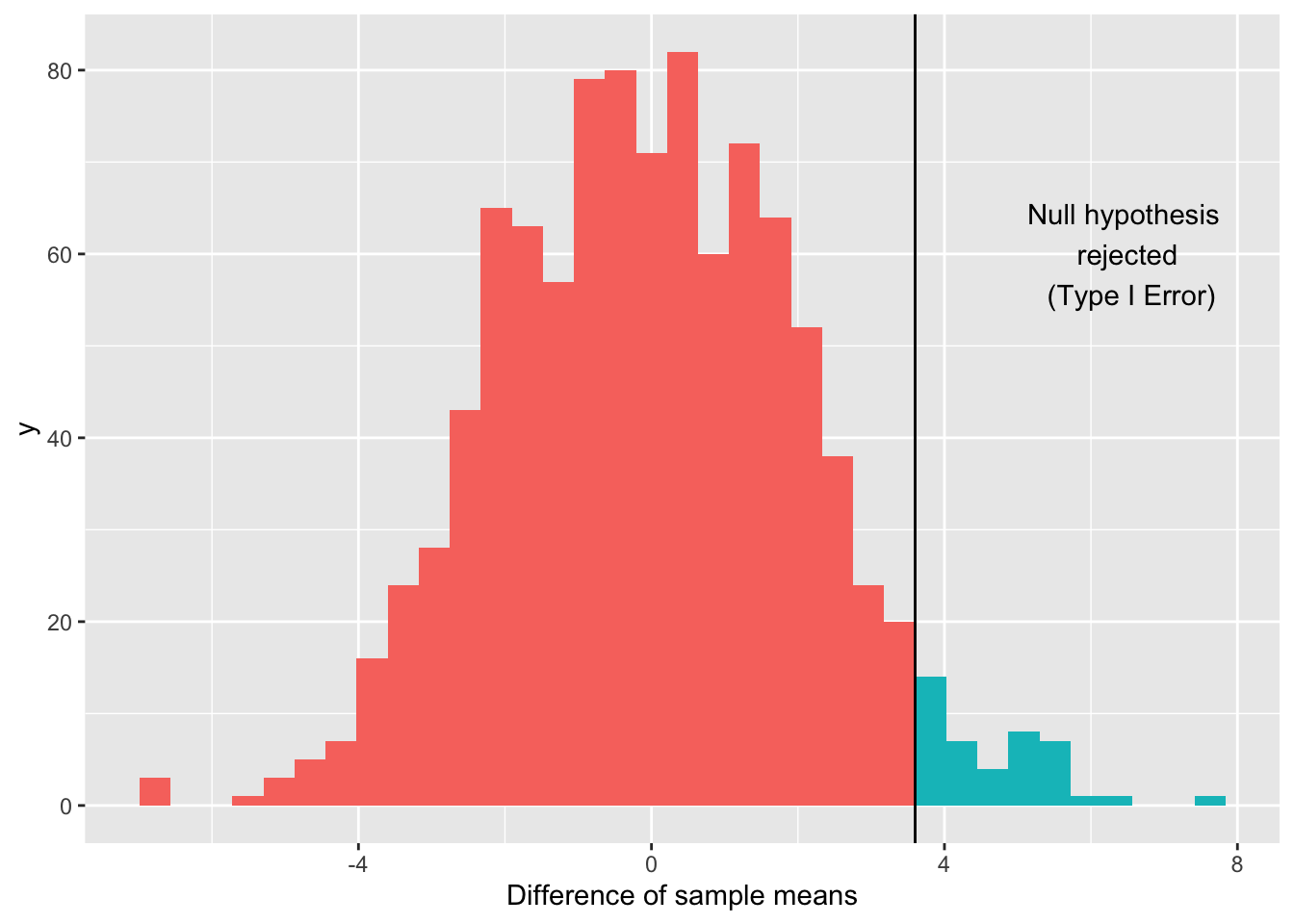
50 out of our 1000 simulations (5% of them) are in the rejection region to the right of the line. In this example, the line falls at $3.46; so any observed differences of sample means falling above $3.46 are times in the simulation when we would have rejected the null hypothesis and been wrong.
When we chose a significance threshold of 0.05, we decided that we are okay with a 5% chance of Type I Error, if in fact the null is true.
12.4.2 Type II Error
What about the studies where we fail to reject the null hypothesis? Are we safe from sampling variability pitfalls? Not quite!
There is also the possibility that our alternate hypothesis was in fact correct, but alas, the data we collected did not lead us to evidence for this fact. We call this situation Type II Error.
Type II Error can occur for a few different reasons:
Luck of the sample. Just as sampling variability can lead us to Type I Error, we can also get back luck in the other direction. What if our waiter had happened to observe tables in a week where big spenders came in at lunch? He might have concluded that lunch and dinner have the same average bills, and failed to reject the null.
Small sample sizes. Imagine that instead of sampling 57 tables, our waiter had sampled only one lunch and one dinner table. Even if the bill difference had been very large - say, $20 difference - we would not have much evidence for a true difference of means. There is just too much uncertainty in our one-observation samples (with standard deviations of $10.03 for dinner bills and $5.00 and lunch bills) for us to reach much of a conclusion. We would never reject the null hypothesis, even if it were indeed false.
Small true differences. Perhaps it is true that dinners cost more than lunches on average, but the true mean difference is only $0.10. This difference is definitely not equal to zero - so the null hypothesis is false. However, we would have to observe a huge number of observations to be able to detect a difference that small and reject the null.
When designing a study, it is good to think about the power of that study: how often will the study successfully avoid Type II Error? A study with high power has a very low probability of Type II Error occurring; a study with low power, like the one-observation example, will commit Type II Error very often.
Calculating the power of a particular experiment or study is complicated, and beyond the scope of this book. However, we will make sure to think about power on a high level, and to remember that Type II Error was possible any time we failed to reject the null hypothesis.