6 Sampling variability
Sampling variability and standard deviation
“If you’re one in a million, and the world is full of seven billion people, that means there are seven thousand people just like you.”
― Jeff Goins
Consider the following study:
An employee claims that his salary of $80,000 is lower than the average salary for his position at other companies. To prove this, he reaches out to employees with the same job at five other companies. He finds that the average salary of these five people is $82,000. “Ah-ha!” he concludes, “I’ve proven my point!”
Do you think that the employee made a strong case for a raise? It’s certainly true that the average from the other companies was $2000 higher, and that’s not a small amount of money! But do we know for sure that our hero has a salary below the true average across all companies?
If you are a bit skeptical of the strength of his conclusion, your instincts are already serving you well. For example, maybe at the five companies he sampled, four employees had salaries of $70,000 and one had a salary of $130,000, leading to a mean of $82,000; in this case, he hasn’t really proven that his salary should be higher!
On the other hand, suppose he finds the average salary of the other five employees to be $150,000. Certainly then, even if those five didn’t all have the exact same salary, it’s pretty clear that our hero should be paid more!
In this unit, we will take a step up from looking only at summary statistics like the mean, and begin using more information to think about the strength of our conclusions.
Recall that we always consider our data to be a sample from a population. Because we only study some subset of all the possible cases, we can ask ourselves, What would have happened if we’d gotten a different sample?
Suppose you and I want to figure out the average height of people in our town. You find 10 random people off the street, and I do the same. Is it likely that we happen to survey the exact same 10 people? Of course not!
That means that in your dataset, you will have different values for the variable Height than I will in my dataset. We are both trying to estimate the parameter true average height of people in this town, and we are both planning to estimate it using the sample mean of our observed values. However, because we happened to sample different sets of people, we will probably end up with slightly different estimates!
Of course, this doesn’t mean our estimates totally disagree. If your estimate was more than a foot taller than mine, we’d be pretty darn surprised! It’s not impossible that this could happen: maybe the first 10 people I find are all below 5 feet tall, and the 10 people you chose are above 6 feet tall. This would be absurdly bad luck - but as long as our town is large enough to have at least ten extra-short folks and ten extra-tall folks, it could happen.
Although it’s possible for such an extreme disagreement to happen by luck, it’s not probable. It’s far more likely that you and I both find a couple short people, a couple tall people, and few in the middle. While we probably won’t calculate the exact same sample mean, we’d reasonably expect our answers to be close, and to both be pretty good guesses about the true mean.
The principle in the scenario we just imagined is called sampling variability: we can never know for sure that we didn’t get an unlucky random sample, but we have some idea of how likely or unlikely particular results might be.
6.1 Quantifying Variability
To learn how to quantify our sampling variability, let’s begin by focusing on a sample of only one observation. If, instead of sampling 10 people from our town, you and I each randomly chose only one person - what might we see?
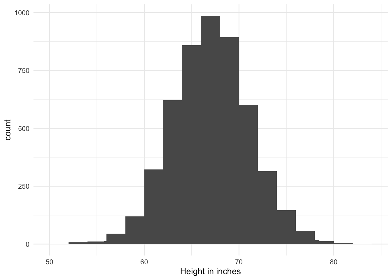
If we knew the heights of every person in our town, we could easily answer that question. For example, maybe our town has 5000 people in it, and a histogram of all their heights looks like this:
What are the chances that the one person I sample has a height below 5 feet (60 inches)? And what are the chances that the one person you sample has a height above 6 feet (72 inches)?
We can estimate these probabilities from our histogram:
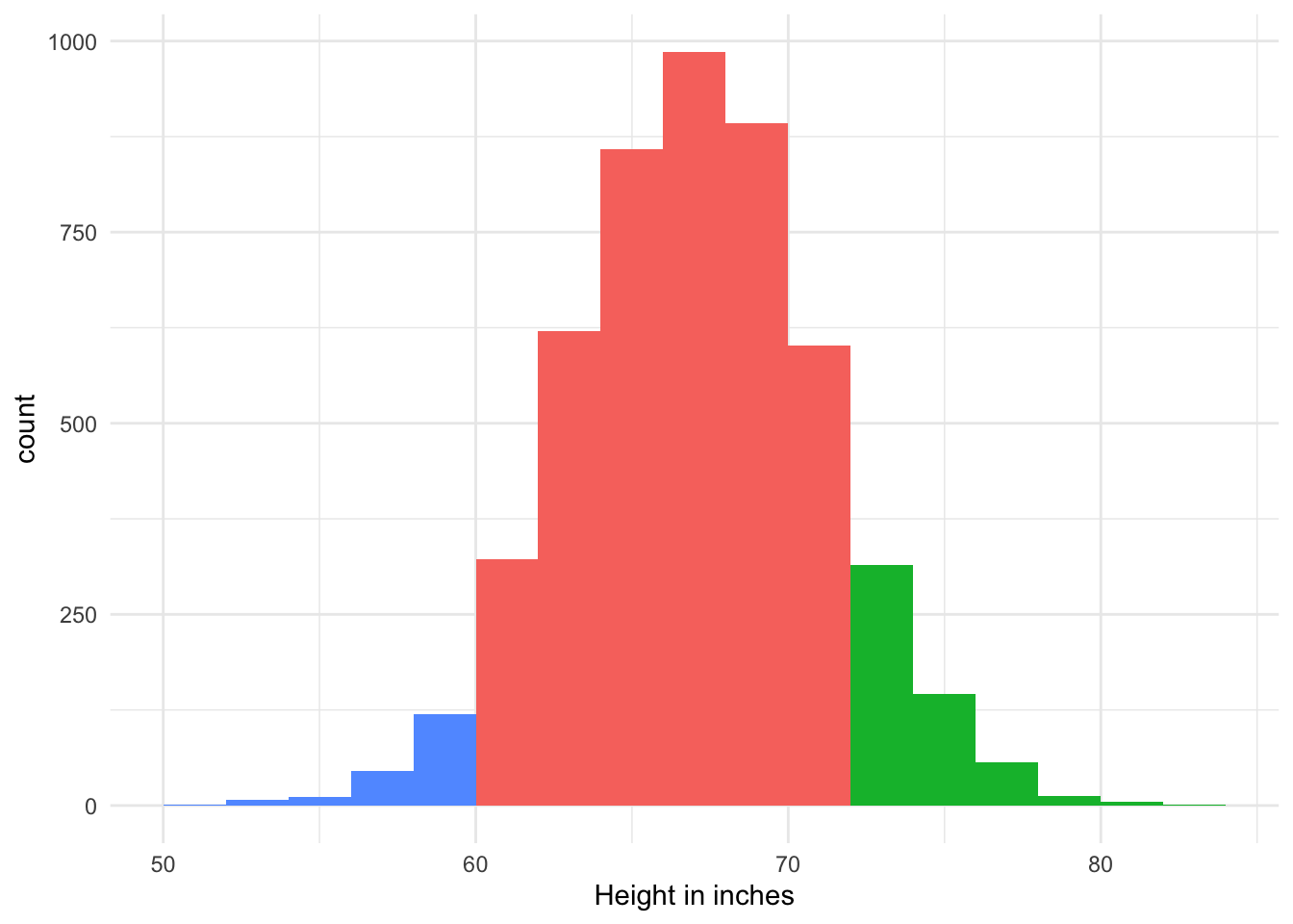
Perhaps we might estimate that there is a 5% chance of randomly choosing someone under 60 inches, and a 10% chance of choosing someone above 72 inches.
But wait - if we knew everyone’s heights in our town, we’d already know the true mean height, and we wouldn’t need to be sampling people at all!
Without access to the whole population, how can we get an idea of what is possible and what is probable in our one-observation sample?
6.1.1 Standard Deviation
While we don’t know every single person’s height in the town, we have some sense of the range of typical human heights. We’ve probably met a few people below 5 feet tall and several above 6 feet tall; we may even have met people below 4 feet or above 7 feet! Most people we encounter are probably somewhere in the middle, around 5’4” to 5’10” or so.
In other words, we can think about how far from the average height people tend to be. This quantity - the typical distance from the mean that we might expect to see in a random observation - is called the standard deviation. (You can think of this as, “What is the standard amount that a person’s height might deviate from the overall mean?”)
Thinking about people’s heights, we might say that the true mean is probably around 5’7” (67 inches). It is very uncommon to find a person more than 1 foot (12 inches) above or below this mean. It is somewhat uncommon to find a person more than 6 inches above or below the mean. It is quite common to find people in the 5’4” to 5’10” range, 3 inches above or below the mean. Therefore, we might decide that the standard deviation of human heights is around 3-6 inches.
6.2 Standardization
Okay, so we have guesstimated that the standard deviation of human heights is, let’s say, around 4 inches.
How does this help us determine what we might see in our sample of size one?
One thing we can now do is describe the observed height of a person in terms of number of standard deviations from the mean. If I sample a person who is 5 feet tall, that person is 7 inches shorter than 5’7”, so they are (7 inches divided by 4 inches = ) 1.75 standard deviations below the mean.
If you sample a person who is 6 feet tall, that person is 5 inches taller than 5’7”, so (5 inches divided by 4 inches equals) 1.25 standard deviations above the mean.
Thus, we can say that my sample was more “unlucky”, or more extreme than yours!
This calculation is called the standardized score or z-score. In general, it is computed as follows (with “standard deviation” abbreviated to “SD”):
\text{z-score} = \frac{ \text{observed value} - \text{presumed parameter}}{\text{SD of observed value}}
In addition to allowing us to compare two values - like my 5 foot tall person and my 6 foot tall person - the standardized score gives us a rough idea of how often we should expect to see that value in a random observation. A value that has a z-score of 3 is approximately 3 standard deviations from the mean, so that value is very uncommon in the population. A value with a z-score of 0.5, on the other hand, is less than one standard deviation from the mean and thus is not at all rare.
Note
In the above, we are using vague terms like “not very rare” or “quite uncommon” to describe the possible values in our sample. In general, we can’t say much more specific than that, since we don’t know all of the true values in the whole population.
Later in this course, we will learn how to use information about the mean standard deviation to be more specific about the values we expect.
6.3 Sample size and uncertainty
We’ve just seen how the standard deviation gives us an idea of the range of values we might reasonably expect when you and I each sample one person and ask their height.
Now let’s return to the original version of the study, where you and I each sample 10 people and record all of their heights. We have an idea of the variability for each of those 10 heights - but that’s not really what we are interested in. Our purpose in measuring these 10 heights is to better understand the true mean height of all people in our town. We will use the sample mean of our 10 heights to estimate this parameter.
Thus, we are no longer wondering what could happen with each individual observation; we are wondering what could happen with our sample mean.
In other words, instead of estimating the standard deviation of a person’s height, we now want to estimate the standard deviation of the sample mean of 10 heights.
You probably already have some instinct for how these two concepts are related. Which of the following do you think is more likely to be a good guess about the true mean height in our town?
- A sample of one person’s height
- The sample mean of 10 people’s heights
- The sample mean of 100 people’s heights
Hopefully, it feels obvious that the third approach would be the best. But what do we mean by “best”? We can think of “best” as “less likely to result in an extremely wrong guess”. It’s certainly possible that a sample of one person happens to select someone of exactly average height, while the sample of ten unluckily selects ten shorter-than-average people. But which sample is more likely to get unlucky? Of course, it’s much more common to find one shorter-than-average person than ten; and finding ten is more common than finding a hundred!
Our natural instinct for “more samples is better” is actually directly related to the standard deviation of the sample mean - i.e., how far we think a sample mean will usually fall from the true mean.
So, returning to our question: Which do you think will be smaller,
- The standard deviation of one person’s height
- The standard deviation of the sample mean of 10 people’s heights
- The standard deviation of the sample mean of 100 people’s heights
Hopefully, you again chose the third option! While all three approach could land close or far from the true mean, the third option is most likely to land closer: the typical amount that the third sample mean will deviate is smaller.
It turns out that there is a straightforward math rule that tells us exactly how much smaller the standard deviation of the sample mean is for larger sample sizes:
\text{SD of sample mean from } n \text{ samples} = \frac{\text{SD of one observation}}{\text{square root of } n}
We guessed that the standard deviation of one person’s height was around 4 inches. Therefore, we might guess that the standard deviation for our sample mean of 10 heights is:
\frac{4}{\sqrt{10}} = 1.26
When I sampled one person and found their height to be 5 feet (60 inches), I was was not that surprised - it was only 1.75 standard deviations below our assumed true mean, after all.
But if I sampled ten people and found an average height of 5 feet, I would be very surprised! The z-score for this sample mean is
\text{z-score} = \frac{60 - 67}{1.26} = -5.56
which tells me that a value of 60 inches is over five standard deviations below the true mean ! That is a very unlucky sample!
6.3.1 Notation
In this course, I encourage you to use words rather than symbols whenever possible. However, there are some common symbols that you will see “in the wild”, and that can provide handy shortcuts for your notes if you get used to them.
Here are a few to know for now:
x = The value of one observation, e.g. one randomly sampled person’s height.
n = The number of observations in a sample.
\bar{x} = A sample mean from a sample of many observations, e.g., the mean of ten people’s heights.
s_x = The standard deviation of one observed value.
s_{\bar{x}} = The standard deviation of a sample mean.
\mu = The true mean. Typically, you will see Greek letters used to represent parameters. This one is written “mu” and pronounced “mew” - you can remember it because it is a Greek “m” to stand for “mean”.
Using this notation, we can rewrite a few of our recent calculations:
\text{z-score of }x = \frac{x - \mu}{s_x} = \frac{60 - 67}{4} = -1.75
s_{\bar{x}} = \frac{s_x}{\sqrt{n}} = \frac{4}{\sqrt{10}} = 1.26
\text{z-score of } \bar{x} = \frac{\bar{x} - \mu}{s_{\bar{x}}} = \frac{60 - 67}{1.26} = -5.56
Notice how the top and bottom of the two z-score equations match: When we want to measure how far x is from \mu, we measure it in terms of s_x; and when we want to measure \bar{x}, we use s_{\bar{x}}.
6.4 Answering research questions
One aspect of the above examples that might strike you as strange is: If we already are willing to assume that the true average height of humans is 67 inches, why are we bothering to estimate the average in our town?
Indeed, this study would be nonsense if we believe the people in our town have the same true average height as the one we already know. But maybe we have a more nuanced research question: maybe we think that residents of our town are, on average, particularly short compared to typical humans.
In other words, there are two proposed facts about our town, which can’t both be true:
- The average height in our town is 67 inches, just like everywhere else.
- The average height in our town is shorter than 67 inches.
Is our data compelling enough to support Fact 2 over Fact 1?
If we took a sample of one person, and saw their height to be 5 feet tall, probably not. Although this person is certainly shorter than average, it’s not surprising to find one short person, by chance, in a typical population. The z-score of -1.75 tells us that this result is not very uncommon even if the true mean height is 67. There’s no real reason to disbelieve Fact 1.
But from our sample of 10 people, if we see a sample mean height of 5 feet tall, perhaps we’ve made a stronger case for Fact 2. The z-score of -5.56 tells us that this result is very unlikely to occur if we are sampling from a population with a mean height of 67. For Fact 1 to be true, we’d have to have gotten very unlucky with our sample! Perhaps a better explanation for what we saw in the data is that Fact 2 is the true one.