7 2.1 Exercises
7.1 Exercise 2.1.1
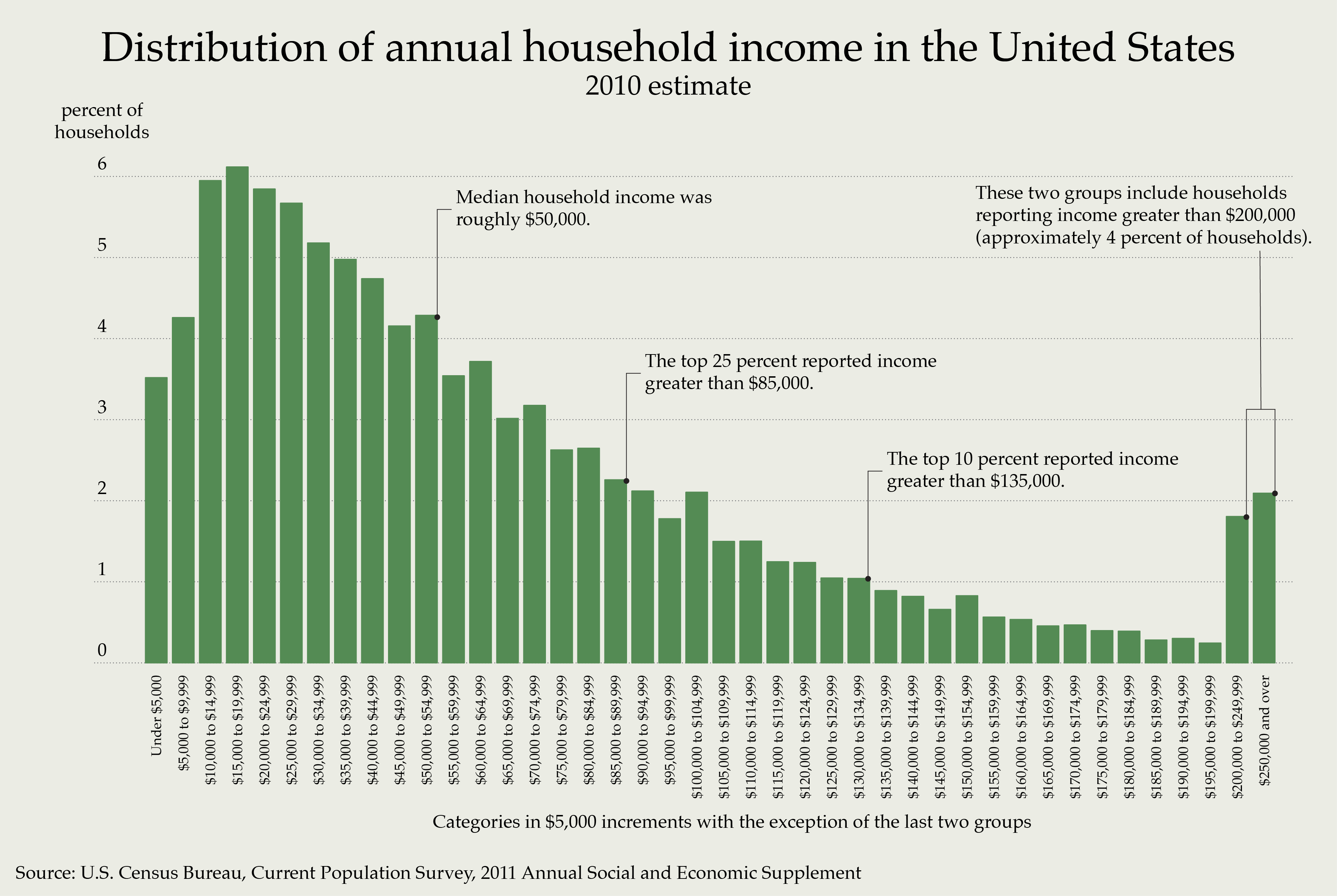
Consider the following histogram, which shows the distribution of annual household incomes in the United States in 2010.
- Visualization and Skew
Notice that this histogram is not quite a true histogram, because the bin width of the last two bins is different from the rest. This is because the distribution of income is extremely right-skewed, and it would not fit on the page if it were constructed properly.
If you are looking at this image on a typical computer screen or a regular sized sheet of paper, the distance from $0 to $100,000 on the x-axis is probably about 4 inches.
In 2010, the world’s richest man, Microsoft Founder Bill Gates, increased his net worth by about $40 billion dollars. (Source: Forbes Rich List)
Suppose you wanted to draw this histogram with all the bins the same width, so that the x-axis extended all the way to $40 billion ($40,000,000,000). How long would that x-axis need to be?
(Hint: $40 billion is 40000 times $100,000. There are 12 inches in a foot, and 5280 feet in a mile.)
- Suppose you randomly choose a household in the United States. For each of the following possible outcomes, state whether you think it is likely, possible but unlikely, almost impossible, or completely impossible.
- An observed income of -$40,000.
- An observed income of $0.
- An observed income of $40,000.
- An observed income of $75,000.
- An observed income of $150,000.
- An observed income of $4 million.
- An observed income of $40 billion.
- Suppose you randomly choose ten households in the United States. For each of the following possible outcomes, state whether you think it is likely, possible but unlikely, almost impossible, or completely impossible.
- A sample mean income of -$40,000.
- A sample mean income of $0.
- A sample mean income of $40,000.
- A sample mean income of $75,000.
- A sample mean income of $150,000.
- A sample mean income of $4 million.
- A sample mean income of $40 billion.
7.2 Exercises 2.1.2
Colleges in the United States have historically used two standardized tests to measure student abilities: the SAT (Scholastic Aptitude Test) and the ACT (American College Testing).
The SAT is designed so that the mean score of all students in a given year is 1100, with a standard deviation of 200.
The ACT is designed so that the mean score of all students is 20.8, with a standard deviation of 3.
- The following table shows the scores for a few students applying to college.
Student | Exam | Score |
|---|---|---|
Samus | SAT | 1245 |
Yoshi | ACT | 31 |
Donkey Kong | ACT | 22 |
Link | SAT | 1580 |
Peach | SAT | 1370 |
Calculate the standardized score for each student.
- Suppose you are in charge of giving out a prestigious scholarship, that only goes to students with remarkably high scores on the SAT or ACT. Do any of these students deserve the scholarship? Make an argument based on the z-scores.
7.3 Exercises 2.1.3
Let’s continue studying the ACT and SAT. Now, we will study schools instead of individual students.
In the table below, we see the names of five high schools, and the corresponding sample mean from a random sample of students at that school.
High School | Number of Students | Exam | Mean Score |
|---|---|---|---|
Zebes Academy | 12 | SAT | 1245 |
Island High School | 1 | ACT | 31 |
Congo High School | 180 | ACT | 22 |
Hyrule Academy | 5 | SAT | 1580 |
Royal Academy | 16 | SAT | 1370 |
Calculate the standard deviation of the sample mean for each school.
Calculate the z-scores for each school’s sample mean.
7.4 Exercises 2.1.4
(Continue the scenario from Exercises 2.1.3)
The school board would like to give an award to the school with the most impressive SAT/ACT scores. For which school do we have the strongest argument, based on the data, that the students achieve higher-than-average scores?
Explain why the answer to #2 is not the school with the highest score on the relevant exam.