Game | Player | Time | Coins | Won |
|---|---|---|---|---|
1 | Maria | 5.41 | 1 | No |
2 | Maria | 12.75 | 7 | Yes |
3 | Maria | 10.66 | 0 | No |
4 | Maria | 15.61 | 8 | No |
5 | Maria | 11.12 | 3 | No |
6 | Maria | 15.99 | 5 | No |
7 | Maria | 16.17 | 13 | Yes |
8 | Maria | 10.69 | 5 | No |
9 | Maria | 9.45 | 14 | Yes |
10 | Maria | 16.88 | 5 | No |
11 | Luisa | 15.02 | 7 | No |
12 | Luisa | 16.01 | 15 | Yes |
13 | Luisa | 11.59 | 3 | No |
14 | Luisa | 8.31 | 9 | No |
15 | Luisa | 6.74 | 14 | No |
16 | Luisa | 13.49 | 17 | Yes |
17 | Luisa | 13.63 | 8 | Yes |
18 | Luisa | 23.85 | 33 | Yes |
19 | Luisa | 13.81 | 17 | Yes |
20 | Luisa | 13.17 | 21 | Yes |
Fictitious dataset of 'Super Sisters' video game sessions by two imaginary players. | ||||
2 Counts and percentages from categorical variables
Basic summaries of data
“At the center of your being you have the answer; you know who you are and you know what you want.”
- Lao Tzu
The following dataset, which records 10 each games of a particular video game called Super Sisters, played by two players named Maria and Luisa. For each game, we have written down:
- how long the player took to play the game, in minutes;
- how many points the player earned; and
- whether or not the player won that game.
Every time we encounter a new dataset, it is a good idea to start by establishing the cases/observations and variables. In this dataset, the cases are unique times someone played the game. These cases are indexed by the Game variable. There are 20 observations.
We have four variables in this dataset: Player, a categorical binary variable which tells us who was playing; Time, a continuous quantitative variable indicating how long (in minutes) the game lasted; Coins, a discrete quantitative variable which tells us how many coins (points) the player gathered in the game; and Won, a binary variable telling us if the player achieved the game goal or not.
Our goal will be to study this game and answer the following research questions:
How often do players tend to win this game?
How many coins do players usually earn when playing this game?
How long does this game take to play?
Consider the question How often do players tend to win this game? The variable in our dataset that can answer this question is the Won variable. We would like to come up with a summary of this variable that provides a reasonable answer to the question.
The first type of summary that we make for categorical variables is called a frequency table. This tells us how many observations fell into each category of the variable, i.e., the counts of the variable.
Won | n |
|---|---|
No | 11 |
Yes | 9 |
You may also sometimes see frequency tables displayed in wide form, like this:
No | Yes |
|---|---|
11 | 9 |
This frequency table supplies a good summary of what is going on in our dataset: of the twenty games observed, 11 ended in losses and 9 ended in wins. Unfortunately, it doesn’t really address the target question. If someone asked you, “How often to people tend to win at Super Sisters?”, would you answer “Nine!” Of course not.
Typically, a research question is a question we ask about general trends, which we answer using some specific data. In this case, the question is asking about what we should expect to happen when anyone plays Super Sisters, not about what happened in the 20 games we observed.
A better summary of our Won variable would be something we can generalize to contexts outside what was directly measured in our dataset. For categorical variables, that means we want to know the percent of the observed data that fell into each category.
In this case, we have:
- 11/20 = 55\% of our observed games were losses
- 9/20 = 45\% of our observed games were wins
We could also simply include percentages in our frequency table:
Won | n | percent |
|---|---|---|
No | 11 | 0.55 |
Yes | 9 | 0.45 |
Now, we have a reasonable way to answer “How often to players tend to win Super Sisters?” - we would say that players probably win about 45% of the time. In other words, you are about as likely to win as you are to lose, with perhaps a bit higher chance that you lose.
2.0.0.1 Communicating your results
Notice that when we reported the percentages above, we said “55% of our observed games were losses”, not “55% of the Won variable fell into the No category.”
Technically, both are correct, of course - a value of No in the Won category is the same as saying that the game recorded in that row of the dataset was a loss.
However, it’s our job as Data Scientists to communicate our results in a way that is clear, to the point, and accessible to all. We’d like to report our conclusions in real-world context, so that a person who hasn’t actually seen the collected data could still understand the takeaway message.
2.1 Measures of center for quantitative variables
Now consider the question, How many coins do players tend to earn when playing this game?
If we list out the values of the variable Coins, we get:
1, \; 7, \; 0, \; 8, \; 3, \; 5, \; 13, \; 5, \; 14, \; 5, \; 7, \; 15, \; 3, \; 9, \; 14, \; 17, \; 8, \; 33, \; 17, \; 21
It’s a bit hard to get a sense of a typical value from this list, but perhaps things will be clearer if we put the numbers in order:
0,\;1,\;3,\;3,\;5,\;5,\;5,\;7,\;7,\;8,\;8,\;9,\;13,\;14,\;14,\;15,\;17,\;17,\;21,\;33
This is a bit better! Now, how can we use this list of numbers to come up a good summary statistic? What one number would be the best answer to the question, “How many coins to players tend to get in a game of Super Sisters?
There are a few different options we might use.
2.1.1 The Mode
One way to measure the “typical” number of coins is to ask, “What was the most common value for the Coins variable in the observed data?” This measurement is called the mode. In this data, we see that the value 5 occurred the greatest number of times (three times). Thus, we might answer the question, “What is a typical score for Super Sisters?” by saying, “The mode of the observed scores is 5.”
Is this the best way to answer to the question? Does the fact that the exact number 5 was the most common make it the ideal summary for the Coins variable? Not really. We saw the mode of 5 happen three times, but we also saw many scores happen twice (3, 7, 8, 14 and 17). In this data, the number 5 doesn’t stand out as particularly important.
So, why is the mode a measurement that is defined in data analysis? In Chapter 1.4, we’ll talk a bit more about the mode of quantitative variables.
For the question we are trying to answer now - “What is a typical score?” - we’d rather choose a measure of center for the Coins variable.
2.1.2 The Median
We can see that the lowest score, which we call the minimum, was 0; and the highest score, called the maximum, is 33.
So, what value represents the center of this list of numbers? It might be tempting to say that the middle is halfway between the minimum and the maximum:
\frac{33 - 0}{2} = 16.5
However, this doesn’t quite match what we saw in the data. If we look at the twenty games played by Maria and Luisa, only four of them had scores higher than 16.5. Is it really reasonable to say that 16.5 is the best measure of center of the Coins variable? Probably not.
Instead, maybe we want to think of the “middle” as the value such that: Half of the observed games scored higher than this number, and half the observed games scored lower than this number.
Looking at the values, we can see that the list is split in half, with ten observed games on each side, between the two observations of 8 coins.
0,\;1,\;2,\;3,\;3,\;5,\;5,\;7,\;7,\;8 \;\;|\;\;8,\;9,\;13,\;14,\;14,\;15,\;17,\;17,\;21,\;33
This measure of center is called the median. In other words, we might answer the question, “How many coins to players tend to earn playing Super Sisters?” with
The median number of coins earned in the games we observed was 8.
In many ways, it feels very natural to summarize the center of our Coins variable using the number that is, in the truest possible sense, the “middle” of the observed values. Have you ever heard the joke,
Half the people you know have below average IQ!
Well, if you choose to measure the average using the median, this statement might be true - we could line up everyone you know in order from lowest IQ to highest IQ, and find out which person is right in the middle of the line. That person’s IQ would then be the median value, and everyone below them would indeed be below average!
2.1.3 The Mean
Although the median is a very intuitive measure, it’s probably not the first thing you thought of when you heard the word “average”. Formally, in the statistical world, average is not a specifically defined term; it can refer to any reasonable measure of center for a quantitative variable.
The measurement that most people think of when they hear “average” is actually called the mean. This measure of center is calculated by adding up all the observed values, and then dividing by the number of observations:
1 + 7 + 0 + 8 + 3 + 5 + 13 + 5 + 14 + 5 + 7 \;\;\;\;\;\;\;\;\;\; + 15 + 3 + 9 + 14 + 17 + 8 + 33 + 17 + 21 = 205
205/20 = 10.25
You’ve probably encountered examples of the mean in your daily life; for example, when a teacher says “The average exam score was 85,” or when someone giving directions says, “This drive takes an average of 35 minutes”, they typically refer to the mean, not the median.
You might wonder, if the median is truly the “middle”, what is the intuitive reason to consider the mean a reasonable measure of center. One way to think of it is this: Notice that in our observed data, the players sometimes got high numbers of coins, like 21, and sometimes low numbers, like 1. What if, instead, the players had gotten the same number of coins in every single game? To reach the same total coins, 205, we would need for every play of the game to have resulted in 10.25 coins. Thus, you can think of the mean number of coins as the “typical” score - i.e., the score we should expect if every game is exactly the same.
When dealing with a discrete variable, like the number of coins earned, it can seem a bit counterintuitive that the mean value isn’t something we could possibly observe in the data - in the game Super Sisters, it’s not actually possible to get 10.25 coins! It’s important to remember that the mean and median are summaries of the observed data, not actual observed values of the Coins variable.
Therefore, it would be very reasonable to answer the question, “How many coins to Super Sisters players tend to get?” by saying, “The mean of the observed values is 10.25,” or more casually, “Players score about 10.25 coins on average.”
2.1.4 Example: Continuous data
Let’s take a moment to compute the mode, median, and mean of the variable Time. The values observed for this variable, in minutes, were:
5.41,\;12.75,\;10.66,\;15.61,\;11.12,\;15.99,\;16.17,\;10.69,\;9.45,\;16.88, \;15.02,\;16.01,\;11.59,\;8.31,\;6.74,\;13.49,\;13.63,\;23.85,\;13.81,\;13.17
or, in order,
5.41,\;6.74,\;8.31,\;9.45,\;10.66,\;10.69,\;11.12,\;11.59,\;12.75,\;13.17, \;\;\;\;\;\;\;13.49,\;13.63,\;13.81,\;15.02,\;15.61,\;15.99,\;16.01,\;16.17,\;16.88,\;23.85
2.1.4.1 Mode
There is no mode for this variable - which is what we would generally expect from a continuous variable, since decimal values are possible and so it’s unlikely that any two observations would be the exact same number.
We can “fudge it”, so to speak, by rounding our observations to the nearest whole number:
5,\;7,\;8,\;9,\;11,\;11,\;11,\;12,\;13,\;13,\;13, \;14,\;14,\;15,\;16,\;16,\;16,\;16,\;17,\;24
In the rounded data, the mode is 16, so we might reasonably say that the most common values of the Time variable is “about 16 minutes”.
2.1.4.2 Median
Taking the ordered numbers and splitting them down the middle gives:
5.41,\;6.74,\;8.31,\;9.45,\;10.66,\;10.69,\;11.12,\;11.59,\;12.75,\;13.17 \; \; |
\;\; \; \;13.49,\;13.63,\;13.81,\;15.02,\;15.61,\;15.99,\;16.01,\;16.17,\;16.88,\;23.85
Recall that for the Coins variable, the dividing line fell between two observations of 8 coins, so we said the median was 8. In this case, though, the line falls between two different numbers: 13.17 and 13.49. Since we are looking for the “middle” of the list of numbers, we’ll simply take the halfway point between the two:
\frac{13.17 + 13.49}{2} = 13.33
Thus, the median play time of a game of Super Sisters, according to our observed data, is 13.33 minutes.
2.1.4.3 Mean
To find the mean, we generally require the help of a calculator or computer - we wouldn’t want to add up all the values by hand. (Realistically, we’d always use software to find the median and mode as well!)
Using a computer, we find that the sum of all the playtimes for the 20 games in our dataset is 260.35 minutes. We divide this by 20 to get a mean playtime of 13.0175 minutes.
2.1.5 Means and medians of dummy variables
Recall that a dummy variable, or one-hot encoded variable, has the value of 0 or 1 depending on whether a category is “active” in that row. For example, converting the Won variable to dummy variables gives:
Game | Player | Time | Coins | Won | Won_Yes | Won_No |
|---|---|---|---|---|---|---|
1 | Maria | 5.41 | 1 | No | 0 | 1 |
2 | Maria | 12.75 | 7 | Yes | 1 | 0 |
3 | Maria | 10.66 | 0 | No | 0 | 1 |
4 | Maria | 15.61 | 8 | No | 0 | 1 |
5 | Maria | 11.12 | 3 | No | 0 | 1 |
6 | Maria | 15.99 | 5 | No | 0 | 1 |
7 | Maria | 16.17 | 13 | Yes | 1 | 0 |
8 | Maria | 10.69 | 5 | No | 0 | 1 |
9 | Maria | 9.45 | 14 | Yes | 1 | 0 |
10 | Maria | 16.88 | 5 | No | 0 | 1 |
11 | Luisa | 15.02 | 7 | No | 0 | 1 |
12 | Luisa | 16.01 | 15 | Yes | 1 | 0 |
13 | Luisa | 11.59 | 3 | No | 0 | 1 |
14 | Luisa | 8.31 | 9 | No | 0 | 1 |
15 | Luisa | 6.74 | 14 | No | 0 | 1 |
16 | Luisa | 13.49 | 17 | Yes | 1 | 0 |
17 | Luisa | 13.63 | 8 | Yes | 1 | 0 |
18 | Luisa | 23.85 | 33 | Yes | 1 | 0 |
19 | Luisa | 13.81 | 17 | Yes | 1 | 0 |
20 | Luisa | 13.17 | 21 | Yes | 1 | 0 |
Although Won is clearly a categorical variable, we have use it to make two quantitative variables instead. Does this suggest that we can take the mean and median of the new dummy variables?
Let’s think about what this looks like. If I add up all the values of Won_Yes, I get:
0+1+0+0+0+0+1+0+1+0+0+1+0+0+0+1+1+1+1+1 = 9 In other words, adding up all the values of the dummy variable Won_Yes gives us the count of the category Yes.
Then, if we divide by the number of observations (20) to find the mean value, we get:
9/20 = 0.45 Voila! The mean value is simply the count of wins divided by the number of games played - in other words, =the percentage for the category Yes in the Won variable.
As for the median, there is less of a satisfying interpretation. We can consider putting the values of the dummy variable in order and finding the middle:
0,\;0,\;0,\;0,\;0,\;0,\;0,\;0,\;0,\;0\;\;\; | \;\;\;\;0,\;1, \;1,\;1,\;1,\;1,\;1,\;1,\;1,\;1 The median, it seems, is 0. This doesn’t tell us much; only that there are more 0’s in the Won_Yes variable than there are 1’s. In other words, these players won their games less than half of the time.
2.2 Robustness and Skew
I’d now like to call your attention to a very important difference between the summaries of the Coins variable, and those for the Time variable. For the Time variable, we had:
\text{Mean} = 13.02 \text{Median} = 13.33
In the context of playtimes, which range from around 5 minutes to around 24 minutes, these two numbers are very close to each other. The two measures seem to nearly agree on the best choice of “center” for the Time variable.
However, for the Coins variable, we calculated:
\text{Mean} = 10.25 \text{Median} = 8
In the context of game scores, which range from 0 to 33, this is a somewhat noticeable difference. Why did this happen?
2.2.1 Extreme Values
When considering a summary measurement for your data, it’s important to think about what would happen if we observed an extreme value - that is, a value that is very different from the rest of the observations.
For example, let’s suppose that Maria plays one more game of Super Sisters, and she manages to score 1000 coins! Obviously, this value is extremely different from the ones we observed in the 20 games in our dataset.
Let’s think about how the median would change if this new observation added as the 21st row in our dataset:
0,\;\;1,\;\;2,\;\;3,\;\;3,\;\;5,\;\;5,\;\;7,\;\;7,\;\; 8 \; \; \; \; |8| \;\;9,\;13,\;14,\;14,\;15,\;17,\;17,\;21,\;33, \; 1000
In this case, the median is still 8! It didn’t change at all when a new, extreme value was observed.
This tells us that the median is a robust measurement: It does not change (much) when extreme values are present. (We sometimes call this resistant.)
Now, let’s consider the mean with the new observation added:
1 + 7 + 0 + 8 + 3 + 5 + 13 + 5 + 14 + 5 + 7 + 15 \;\;\;\;\;\;\;\;+ 3 + 9 + 14 + 17 + 8 + 33 + 17 + 21 + 1000 = 1205
1205/21 = 57.38
Whoa! That changed a lot - from 10.25 to 57.38. It’s clear that the mean is not a robust/resistant measure.
2.2.2 Skew
While it’s clear that the mean responds to extreme values differently from the median, this doesn’t quite explain the discrepancy we see between the mean and the median in the Coins variable, since there aren’t any notably extreme values.
Instead, we see something a bit more subtle: the values at the lower end are closer together than those at the upper end. To see this, let’s mark our observed values on a number line:
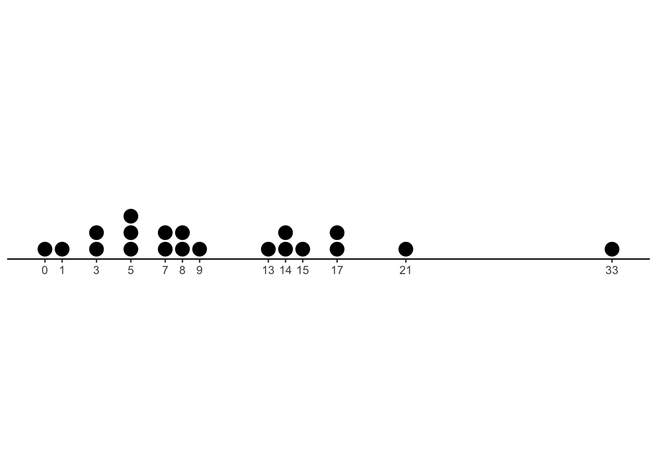
Each dot in the above chart represents one observation from our dataset; for example, in 3 of the 20 games played, the player got 5 coins, and in only one of the games, a player got 21 coins.
What we want to notice here is that there are many observations “bunched” together in the smaller numbers (say, 0-9), but the observations at larger numbers (17, 21, 33) are more spread out. It’s not quite a situation where there is one very extreme value, like 1000; it’s that the distances between values “stretch out” more and more as we move to the right on the number line.
We call this property right skew. (The reverse pattern, where numbers are bunched at the high values and spread out to the left, is called left skew.)
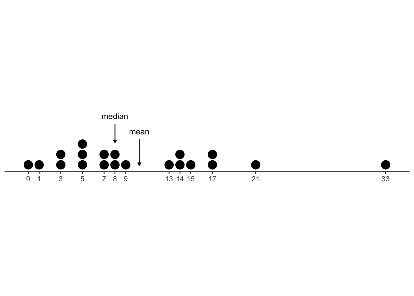
The fact that our variable Coins is right-skewed tells us that the mean will be bigger than the median: The median lives in the “middle” of the values, no matter how spread or bunched they are, while the mean gets “pulled” to the right, towards the far-away higher values. We can see this on the number line below:
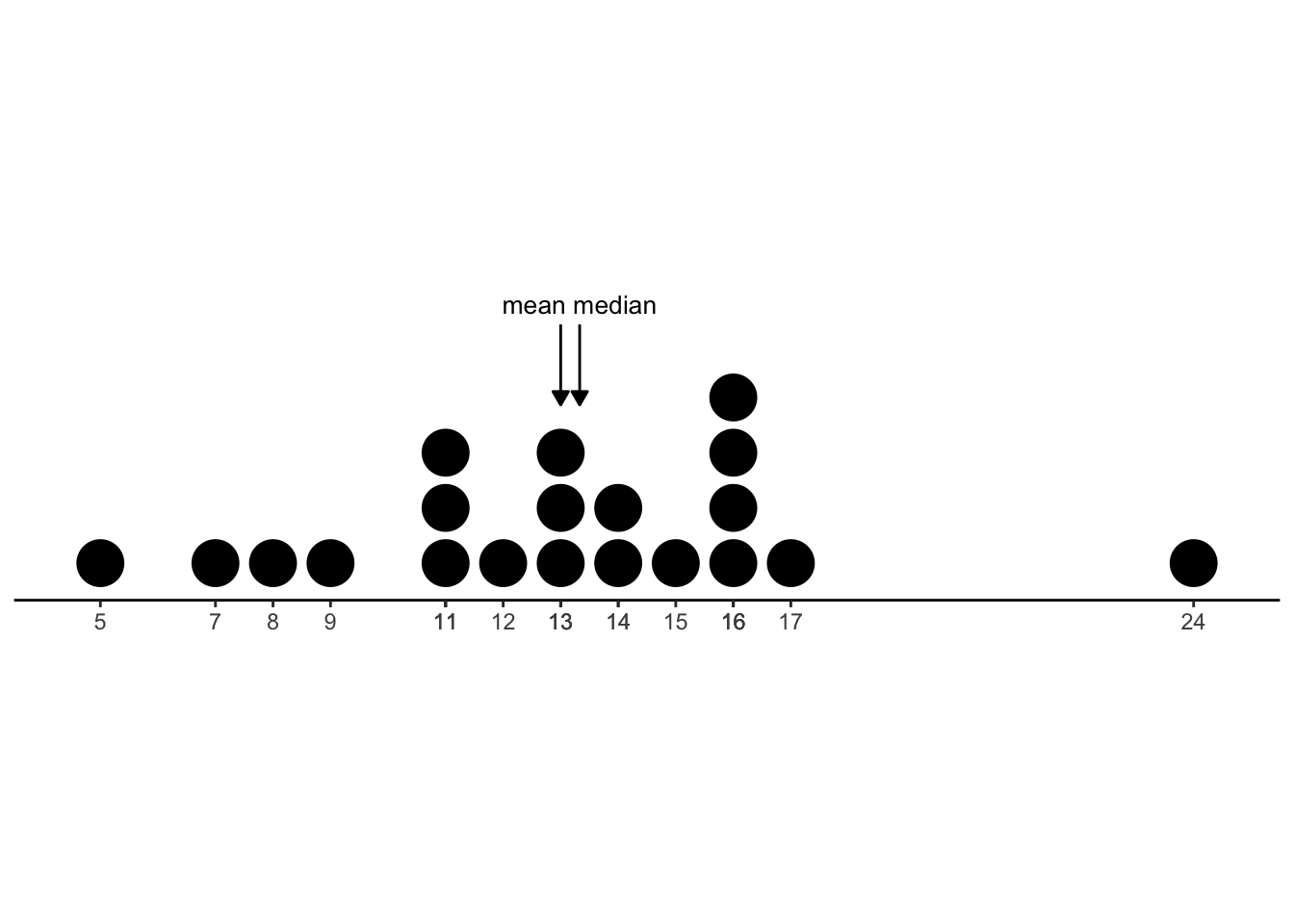
If we look at the Time variable, by contrast, we see that it is neither right-skewed nor left-skewed. (The chart below shows the rounded values of the time variable, to make it easier to visualize.) The values are roughly equally spaced in the high and low ends, and bunched in the middle. When there is no major skew, we call this symmetric. For a symmetric variable, we’d expect the median and the mean to approximately agree.
2.3 Populations and Representative Samples
Something you should be asking yourself right now is, Can this data really answer the research questions? That is, does the context of the dataset indeed reasonably address the questions being asked?
Consider the research question, How often do players tend to win this game?
This question asks about “players” of the game. Have we collected data about all people who ever played Super Sisters? Of course not! We only have data about two players, Luisa and Maria.
Now, it’s not so bad that we don’t have information on all players ever to play this game - that’s an unrealistic goal! Almost all data you will ever analyze is only from a sample, meaning that the observations in the dataset do not represent all possible cases that could exist.
What we really are worried about is whether the sample in our dataset is a representative sample. The goal of our analysis is to make a claim about a population; for example, in our video game analysis, we have identified the population of “players of this video game”.
So, do we believe that Maria and Luisa represent typical players of this video game? Is it reasonable to use data about these two players to arrive at conclusions about all players? Perhaps this dataset is from the Super Sisters World Championships, and Maria and Luisa are the two greatest players ever to play the game. In that case, we certainly wouldn’t expect their results to represent the population of all players! On the other hand, perhaps they are indeed fairly average or “regular” players, and their performance is truly representative. There’s no way to really know without more information.
In Chapter 1.4, you will learn more about how to collect a representative sample from a population.
For now, though, we will modify our research questions so that we only make claims about the population that our sample can reasonably represent.
How often does Maria tend to win this game? How often does Luisa tend to win this game?
How many coins does Maria usually earn when playing this game? How many coins does Luisa usually earn when playing this game?
How long does this game take for Maria to play? How long does this game take for Luisa to play?
2.3.1 Scope and Certainty
We always want to make sure the scope of the conclusions we draw from data is appropriate to the population that the data were sampled from.
Is it reasonable to believe, based on this dataset, that if your grandma plays a game of Super Sisters, she will take around 13.6 minutes to play, and she will get around 14.4 coins? Who knows!
Is it reasonable to believe, based on this dataset, that if Luisa plays another game of Super Sisters, she will take around 13.6 minutes to play and she will get around 14.4 coins? Yes, this appears to be a reasonable guess!
Remember, though, that we are still making broad claims based on only the sample that we get to observe. We don’t know for sure what’s going on in the rest of the population.
Are we absolutely certain, based on this dataset, that if Luisa plays another game of Super Sister, she will take 13.6 minutes to play and she will get 14.4 coins? No way!
2.4 Parameters and Statistics
When we say, How often does Maria tend to win?, we are not asking about what has happened, or what will happen - we are asking something deeper about what kind of player Maria is. We would like to be able to characterize her playing ability by knowing her “true” win percentage.
This value - the “truth” that best describes Maria’s win percentage - is called a parameter. The word parameter refers to a numeric measurement that we can never actually know the value of.
There are a few ways to conceptualize parameters when they are percentages:
2.4.0.1 A percentage of the population
Note that even though we’ve modified our research questions to focus on Maria and Luisa individually, we would still consider our dataset to represent a sample from a population. In this data, we have measured the results of ten games played by Maria. But our research questions implicitly asks about all games Maria has ever played. Do we know that these ten games are all she have ever played? Not necessarily!
Imagine that we had written down all the games of Super Sisters Maria has ever played. Then, we could calculate what percent of all those games were wins.
Although we don’t realistically have access to data for the full population, that doesn’t stop us from thinking about “What if?” We can still say that the parameter of interest is “the percentage of wins out of all games of Super Sisters Maria ever played.”
2.4.0.2 A long-run proportion
Suppose we did know these ten games were all that Maria had ever played. If she played a hundred more games, are you absolutely sure that she would win 30 of them, just because she won 30% of her first ten? Of course not.
Then, perhaps we could regard the population as all games Maria has ever have played or will ever play.
We can’t possibly observe data for events that haven’t happened yet, like Maria’s future games of Super Sisters. Once again, though, we can still conceptualize this measurement. We can say that our parameter of interest is in fact, “The proportion of Super Sisters games that Maria would win if she played many many more times.”
2.4.0.3 The probability of the next time
But wait! Even if she never plays another round of Super Sisters again, are you definitely certain that Maria is best described as a player who wins 30% of the time? Maybe she just had an unlucky day on a few of those first ten games. Maybe if she had played on different days, she would have won those games.
Therefore, maybe we should regard our population as all games Maria could hypothetically have ever possibly played or hypothetically could ever play.
That starts to get a bit strange and abstract, so let’s instead rephrase the question as: How likely is Maria to win any given game of Super Sisters? We can see now that we aren’t thinking specifically about any set of actual games, past or future; instead, we are thinking about Maria’s overall skills.
It would then be reasonable to describe our parameter of interest as: “The percent chance that Maria will win a game of Super Sisters.”
2.4.1 Statistics
We now have three strategies for conceptualizing the idea of the “true” percentage that would answer our question, How often does Maria tend to win?
Alas, none of these is a number that we are actually able to calculate in real life: we don’t have all Maria’s games, we can’t observe future games, and we don’t know how likely she truly is to win.
Should we give up? Of course not! We aren’t entirely in the dark, because we do have some information: the ten games played by Maria that we do get to observe. Our goal is to use this data to make our best guess about the true value of our parameter.
You have now arrived at the vocabulary word that defines a whole field of study. A statistic is a summary measurement calculated from sample data, that is meant to be an estimate for a parameter we are interested in about some population.
2.4.2 Example: Quantitative Variable
Consider now the question, How many coins does Maria tend to get?
What might be the parameter that would answer this question? Let’s practice the three ways to think about parameters:
Summary from population: The mean (or median) coins received from all games Maria has played.
Long-run average: The mean (or median) coin counts we would get if Maria were to play many more games.
Expected next time: The number of coins we would expect Maria to score in her next game of Super Sisters.
Regardless of how we choose to frame our parameter, we need a statistic to estimate it.
If our parameter asks about the mean, a good choice of statistic would be the mean that we calculated from our sample data: 6.1.
If our parameter asks about the median, a good choice of statistic would be the median that we calculated from our sample data: 5.
Henceforth, we will use the phrase sample mean to refer to the actual number calculated from observed data, like 6.1, which is a statistic. We will use the phrase true mean to refer to the unknown parameter, like “The mean coins Maria would score if she played many more games.”
Similarly, we will use sample median and true median; sample proportion and true proportion; and so forth, to differentiate statistics from parameters.