Day of Week | Hours of Sleep | Number of Coffees | Breakfast |
|---|---|---|---|
Sun | 9 | 0 | Cereal |
Mon | 7 | 3 | Cereal |
Tue | 4 | 4 | Muffin |
Wed | 10 | 2 | None |
Thu | 5 | 5 | Cereal |
Fri | 8 | 0 | None |
Sat | 6 | 1 | Cereal |
9 Association between a categorical variable and a quantitative variable
Studying variable relationships
Recall from the previous chapter the morning habits of Lori Bilmore:
In this book so far, we’ve learned how to ask questions about one variable, such as:
Is the true probability of Lori eating cereal for breakfast equal to 50%? (Categorical variable: breakfast food)
Is the true mean hours of sleep Lori gets equal to 7? (Quantitative variable: hours of sleep)
But how can we ask questions that involve two variables, such as:
Is Lori more likely to drink coffee on days where she eats cereal for breakfast?
Does Lori tend to get less sleep on days where she eats cereal?
Does Lori drink more coffee on days where she got less sleep?
All of these questions involve studying a relationship or an association between two variables, but they involve different combinations of quantitative or categorical variables. Since these three scenarios require three slightly different ways to approach our questions, we’ll work through them one by one.
Consider the question, Does Lori tend to get less sleep on days where she eats cereal for breakfast?
We know that a summary statistic for a quantitative variable is the sample mean. Thus, if we want to compare across the categories “ate cereal” and “did not eat cereal”, we can separate the cases into those two groups, and find the sample mean of the variable Hours of Sleep in each group:
Day of Week | Hours of Sleep | Number of Coffees | Breakfast |
|---|---|---|---|
Sun | 9 | 0 | Cereal |
Mon | 7 | 3 | Cereal |
Thu | 5 | 5 | Cereal |
Sat | 6 | 1 | Cereal |
Sample mean of Hours of Sleep: 6.75
Day of Week | Hours of Sleep | Number of Coffees | Breakfast |
|---|---|---|---|
Tue | 4 | 4 | Muffin |
Wed | 10 | 2 | None |
Fri | 8 | 0 | None |
Sample mean of Hours of Sleep: 7.3
Clearly, these two sample means are not exactly the same. In fact, we can combine these into one summary statistic that addresses our question: the difference of sample means
\bar{x}_{C} - \bar{x}_{NC} = 6.75 - 7.3 = -0.55
(Recall that \bar{x}_C is our shortcut way of writing “The sample mean hours of sleep one days she had cereal,” and \bar{x}_{NC} is the sample mean for no-cereal days.)
Okay, so in this data we can say that she got, on average, 0.55 less hours of sleep on days where she had cereal for breakfast.
Does this mean that Lori definitely wakes up earlier when she wants to eat cereal? Not necessarily!
9.0.1 Do we have evidence?
When we studied a sample mean of one variable, we asked the question, “How far might this sample mean fall from the true mean, just by luck of the sampling variability?” We quantified that uncertainty with the standard deviation of the sample mean.
Now, we wish to study a difference of sample means. Thus, we’d like to know the standard deviation of the difference of sample means.
First, let’s find the estimated standard deviation for the two means in this data:
s_{C} = 1.7, \; \;\;\;\; s_{NC} = 3.1
SD(\bar{x}_C) = 1.7/\sqrt{4} = 0.85 SD({\bar{x}_{NC}}) = 3.1/\sqrt{3} = 1.79
Our “yes cereal” mean sleep estimate has an uncertainty of about 0.85 hours, and our “no cereal” estimate has an uncertainty of 1.79 hours. We saw a difference of means of -0.55. Does this seem to be a big difference compared to the variability in our estimates? Not really! It’s much smaller than either of the two standard deviations, so it’s very plausible to think that we just saw the difference due to luck.
9.0.2 Standard deviation of a difference of means
Although it seems clear that we don’t have much evidence for a true difference in Lori’s average sleep with and without cereal, let’s calculate an exact standardized statistic.
If our observed difference of -0.55 hours is just due to luck, then Lori really doesn’t sleep differently depending on her cereal plans, so the true difference would be equal to 0.
Thus, a standardized score for the difference of sample means would be:
\text{z-score} = \frac{\text{statistic} - \text{proposed parameter}}{\text{SD of statistic}} = \frac{-0.55 - 0}{\text{SD of difference of means}}
We know that the standard deviations of the two individual sample means are 1.79 and 0.85. Do you think that the standard deviation of the difference of means should be:
- Bigger than 1.79 and 0.85?
- Somewhere between 1.79 and 0.85?
- Smaller than 1.79 and 0.85?
Perhaps a better way to ask this question is: Do you think that making a guess involving two sample means is:
- More uncertain than guessing about only one?
- About the same uncertainty as guessing about only one?
- Less uncertain than guessing about only one?
Hopefully, in the second question, you thought that it was harder to guess two things than to guess just one! In other words, the standard deviation of the difference of sample means should be bigger than either individual standard deviation, because you have more uncertainty.
Mathematically, it turns out that we can add the variances of the two sample means. (Recall that the variance is the standard deviation squared.)
\text{Var}_{(\bar{x}_C - \bar{x}_{NC})} = 0.85^2 + 1.79^2 = 3.93
Therefore, the standard deviation of the difference of sample means is:
S_{(\bar{x}_C - \bar{x}_{NC})} = \sqrt{Var_{(\bar{x}_C - \bar{x}_{NC})}} = \sqrt{3.93} = 1.98
So in general, for any two sample means from categories A and B,
S_{(\bar{x}_A - \bar{x}_{B})} = \sqrt{Var_{(\bar{x}_A - \bar{x}_{B})}} = \sqrt{S_{\bar{x}_A}^2 + S_{\bar{x}_{B}}^2}
Now that we have quantified our uncertainty about the summary statistic “difference of sample means”, we can compute our standardized score:
\text{standardized score} = \frac{\text{statistic} - \text{proposed parameter}}{\text{SD of statistic}} = \frac{-0.55 - 0}{1.98} = -0.28
A good summary of this analysis might look like this:
Comparing days where Lori ate cereal with days she did not, we observed a mean difference of -0.55. If there is no relationship between Lori’s sleep and her breakfast choice, we would expect a difference of means of 0. Our observed difference was only 0.28 standard deviations away from what we expected, so we have no evidence of a relationship between sleep and cereal.
9.1 Association between two categorical variables
Now that we have gone through the trouble of figuring out how to study a difference of means, we’ll find that proportions are very similar!
We know that our best summary statistic for a categorical variable is a sample proportion. To look for associations between categorical variables, we’ll simply compare the sample proportions across categories.
Consider our research question
Does Lori have cereal for breakfast on days she drinks coffee?
The following table shows the counts of a new variable called Had_Coffee (yes or no) and the Breakfast variable.
Had_Coffee | Cereal | Muffin | None |
|---|---|---|---|
No | 1 | 0 | 1 |
Yes | 3 | 1 | 1 |
Consider the following two sentences, calculated from the counts above:
When Lori ate cereal for breakfast, she also drank coffee that day 75% (3/4) of the time. When she did not eat cereal, she drank coffee 66% (2/3) of the time.
When Lori drank coffee that day, she ate cereal for breakfast 60% (3/5) of the time. When she didn’t drink coffee that day, she ate cereal 50% (1/3) of the time.
Which of these better answers the question, “Is Lori less likely to get coffee during the day on days she eats cereal for breakfast?” To decide, we want to think about which variable is explanatory and which is response. That is, are we saying that Lori drank coffee because she ate cereal, or that she ate cereal because she drank coffee?
The second version is the more reasonable one in this case. Therefore, we want to condition on the explanatory variable - meaning, we split up the observations into groups using the variable Cereal, and then we compute sample proportions within each group for the variable Had Coffee.
Now, we can see that our two sample proportions, 0.75 and 0.66, are not the same, and we again want to combine these into one summary statistic that addresses our question: the difference of sample proportions
\hat{p}_{cereal} - \hat{p}_{no cereal} = 0.75 - 0.66 = 0.09
9.1.1 Do we have evidence?
Once again, this number by itself does not tell us the answer to our question.
Let’s calculate the standard deviations of the two sample proportions:
S_{\hat{p}_C} = \sqrt{\frac{0.75 * (1- 0.75)}{4}} = 0.22
S_{\hat{p}_{NC}} = \sqrt{\frac{0.66 * (1- 0.66)}{3}} = 0.27
As with the sample means - and indeed, any differences of two statistics! - we can add the variances:
S_{(\hat{p}_A - \hat{p}_{B})} = \sqrt{Var_{(\hat{p}_A - \hat{p}_{B})}} = \sqrt{S_{\hat{p}_A}^2 + S_{\hat{p}_{B}}^2}
\text{Var}_{(\hat{p}_{C} - \hat{p}_{NC})} = 0.22^2 + 0.27^2 = 0.1213
S_{(\hat{p}_{C} - \hat{p}_{NC})} = \sqrt{0.1213} = 0.348
Finally, we can compute a standardized score for our statistic:
\text{standardized score} = \frac{\text{statistic} - \text{proposed truth}}{\text{SD of statistic}} = \frac{0.09 - 0}{0.348} = 0.258
Try to fill in the blanks in the paragraph below to make your conclusion:
Comparing days where Lori ate cereal with days she did not, we observed ___________. If there is ____________ between Lori’s cereal choice and her coffee drinking, we would expect _____________. Our observed difference was _____________ away from what we expected, so we have __________ of a relationship between cereal for breakfast and coffee drinking.
9.2 Association between quantitative variables
Finally, let’s consider the question,
Does Lori drink more coffee on days where she got less sleep?
This question involves two quantitative variables: Number of Coffees and Hours of Sleep.
We could consider simplifying the question by converting the quantitative variable into a categorical variable: We could, as we did earlier in this chapter, change Hours of Sleep to the variable Enough Sleep, by binning into “More than or equal to 7 hours” and “Less than 7 hours”. However, this doesn’t quite address the question completely. 7 hours of sleep is very different from 10 hours - yet we would call both of them “Enough sleep”. Ideally, we’d like to use all the information available to us, and leave Hours of Sleep as a quantitative variable.
So, how do we do this?
9.2.1 Covariance
Recall that when we calculated the variance and standard deviation of one quantitative variable, we measure how far the observed values fell above or below the sample mean.
Let’s do this again, but this time, we’ll do it for both of our variables:
Hours of Sleep | Number of Coffees | Dist from mean Sleep | Dist from mean Coffees |
|---|---|---|---|
9 | 0 | 2 | -2.14 |
7 | 3 | 0 | 0.86 |
4 | 4 | -3 | 1.86 |
10 | 2 | 3 | -0.14 |
5 | 5 | -2 | 2.86 |
8 | 0 | 1 | -2.14 |
6 | 1 | -1 | -1.14 |
We should notice something very interesting in these distances from the means: Most of the times that Lori got less-than-average sleep (i.e. a negative distance), she drank more-than-average coffees (positive distance). The reverse is also true: When she got better-than-average sleep, she usually drank less-than-average coffee.
This tells us something about the association between these variables. It seems that the variability of the observations follows a pattern.
Now consider multiplying the distances together. If one is negative and the other is positive - that is, if they vary in opposite directions for the same observation - we get a negative number. When both are negative, as in the last row, they vary in the same direction (below the mean), and we multiply them to get a positive number.
Hours of Sleep | Number of Coffees | Dist from mean Sleep | Dist from mean Coffees | Multiplied |
|---|---|---|---|---|
9 | 0 | 2 | -2.14 | -4.28 |
7 | 3 | 0 | 0.86 | 0.00 |
4 | 4 | -3 | 1.86 | -5.58 |
10 | 2 | 3 | -0.14 | -0.42 |
5 | 5 | -2 | 2.86 | -5.72 |
8 | 0 | 1 | -2.14 | -2.14 |
6 | 1 | -1 | -1.14 | 1.14 |
We see a lot of negative numbers in the Multiplied column above, which tells us that the variables Number of Coffees and Hours of Sleep seem to follow opposite patterns!
Our last calculation will be to take the average of the multiplied distances, which is called the covariance between the two categorical variables. For these variables, we find a covariance of -2.42.
9.2.2 Correlation
The covariance of -2.42 tells us only one important thing: That the relationship between the variables Number of Coffees and Hours of Sleep is negative. That means that when we see more sleep, we see less coffee; and vice versa.
But, as usual, we’d like to know more. We’d like to quantify exactly how associated our variables are, and we’d like to decide if our data provided strong evidence of a relationship.
The reason that the covariance doesn’t help us much is that it is very dependent on the units of measure in our dataset. Imagine that we did the same calculations as above, but we measured sleep in seconds instead of hours:
Seconds of Sleep | Number of Coffees | Dist from mean Sleep | Dist from mean Coffees | Multiplied |
|---|---|---|---|---|
32400 | 0 | 7200 | -2.14 | -15408 |
25200 | 3 | 0 | 0.86 | 0 |
14400 | 4 | -10800 | 1.86 | -20088 |
36000 | 2 | 10800 | -0.14 | -1512 |
18000 | 5 | -7200 | 2.86 | -20592 |
28800 | 0 | 3600 | -2.14 | -7704 |
21600 | 1 | -3600 | -1.14 | 4104 |
Our calculated covariance is now -8742.86! Yikes. Does this mean that the two variables are much more strongly related than they used to be? Of course not! All we did is change from measuring hours to measuring seconds; we didn’t change anything about the true story behind the pattern in the observations.
We’d like to have a measurement for association that does not change when the units change. If only we had a way to measure the variability, in proper units, of each variable by itself… wait, we do! The standard deviation!
What if we divide the covariance by the individual standard deviations?
With sleep measured in hours, we get:
\frac{\text{covariance}}{\text{(SD of Sleep)}*\text{(SD of Coffee)}} = \frac{-2.42}{2.16*1.95} = -0.57 With sleep measured in seconds, we get:
\frac{\text{covariance}}{\text{(SD of Sleep)}*\text{(SD of Coffee)}} = \frac{-8742.86}{7776.89*1.95} = -0.57
Voila! They are the same number, regardless of which units we use.
This summary statistic, which is commonly used to summarize a relationship between two quantitative variables is called the correlation. We usually represent it with the letter r.
It turns out that mathematically, the correlation is always between -1 and 1. A correlation of -1 is a perfect negative relationship: The more below average one variable is, the more above average we expect the other variable to be. A correlation of 1 is a perfect positive relationship: when one variable is above average, the other will be too; and when one is below average, so is the other. A correlation of 0 represents no relationship or pattern at all.
Thus, our observed correlation of -0.57 shows a moderately strong negative relationship between hours of sleep and cups of coffee.
9.2.3 But do we have evidence?
It’s important not to forget, in all these calculations, that we are still making estimates from the data. Any two quantitative variables have a true correlation, a parameter that we don’t know. (The true correlation is sometimes written \rho, or “rho”, a Greek letter r.)
We’d like to make claims about the true correlation between Lori’s sleep and coffee habits, based on this sample correlation we just computed.
The correlation is a much more complicated calculation than a sample mean - but since it’s an estimate from data, and data has sampling variability, the sample correlation has its own standard deviation!
Rather than compute this from scratch, I’ll give you a shortcut equation:
S_r = \frac{\left(1 - r^2\right)}{\sqrt{n}}
You don’t need to know the math behind this equation, but a two things should not surprise you:
The standard deviation is 0 when the correlation is 1 or -1. If the variables have a perfect relationship - they are always the exact same amount above or below the mean at the same time - there is no variability in their association.
The \sqrt{n} should look familiar: when we estimate anything from more observations, we have more certainty!
In our analysis of Lori’s habits, the standard deviation of our sample correlation is:
S_r = \frac{ 1- (-0.57)^2}{\sqrt{7}} = 0.25
Thus, as usual, we can compute a z-score for the correlation, to see if there is truly a pattern here or if the true correlation is 0:
\text{z-score} = \frac{\text{statistic} - \text{proposed parameter}}{\text{SD of statistic}} = \frac{-0.57 - 0}{0.25} = -2.28
This time, we do seem to have some evidence of an association! Our observed sample correlation was 2.28 standard deviations more negative than what we would expect if Lori’s coffee was not related to her sleep.
Perhaps in this case, we can conclude that Lori drinks more coffee on days when she sleeps less - an unsurprising habit, if a bit unhealthy!
9.3 Scatterplots
When answering research questions, we would certainly like to visualize the data to support our conclusion. How should we approach this in the case of two quantitative variables? We can’t use the color of plot elements, because the quantitative variables could have any value at all, rather than a fixed set of categories.
We know how to plot each quantitative variable individually; for example, we can look at boxplots of Lori’s hours of sleep and number of coffees:
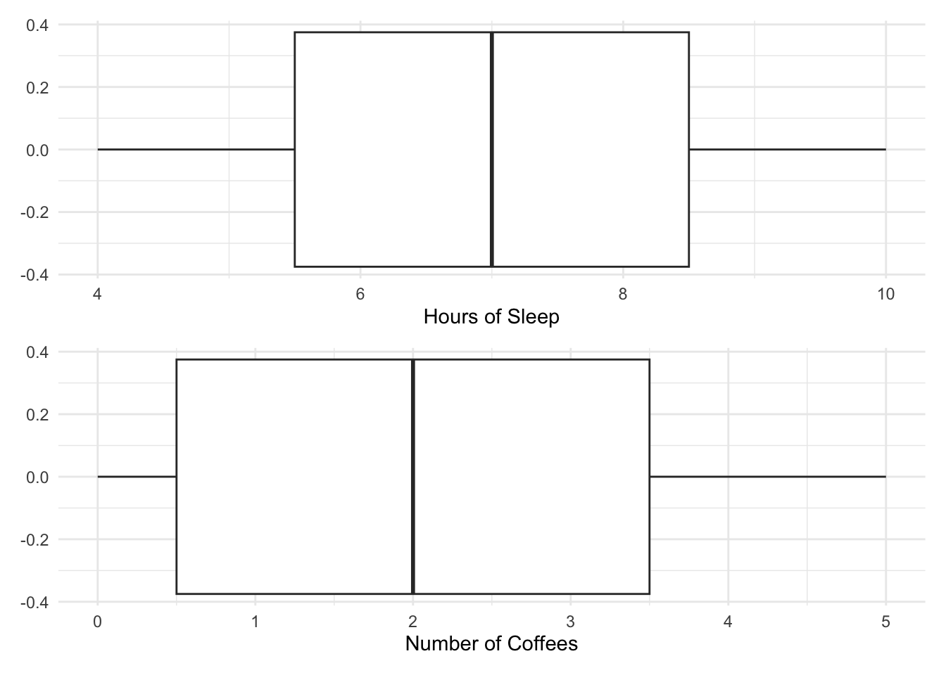
Although these visualizations tell us some things about the variables, like the approximate median, quartiles, and IQR, they do not tell us anything about the relationship between the two variables. This is because we don’t know which values come from the same observation.
To plot two quantitative variables, we think of the observations as being paired. That is, instead of saying the values of Hours of Sleep are (9, 7, 4,…) and the values of Number of Coffees are (0, 3, 4, …) we will say that the observed pairs of values are (9, 0), (7, 3), (4, 4), etc.
We then construct a scatterplot by drawing a dot at each pair:
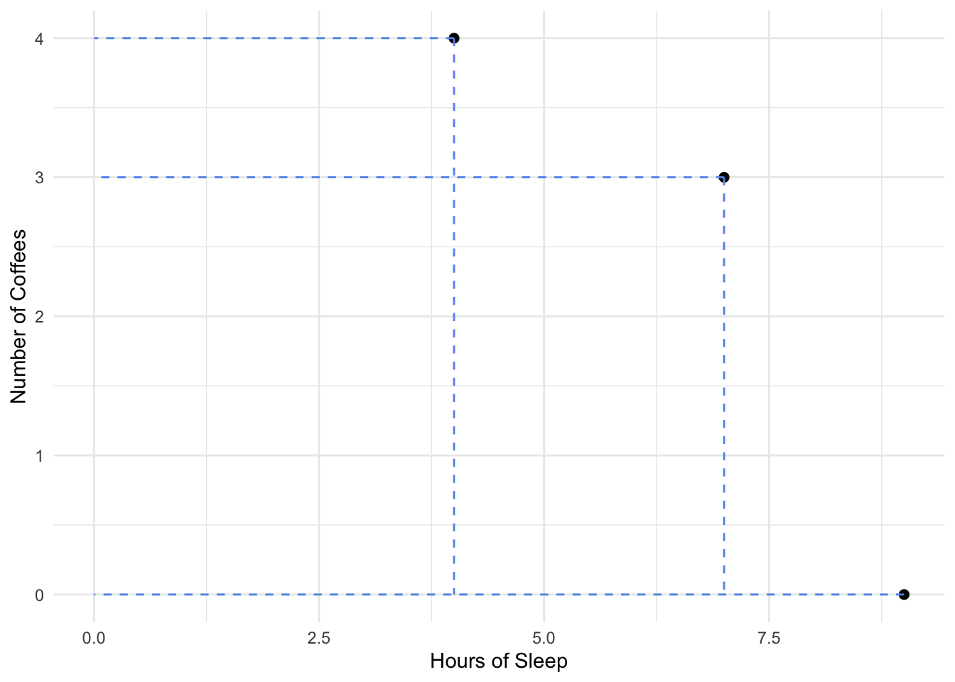
Each point corresponds to one case in our dataset - in this data, one day of the week that we observe Lori. The location of the point on the x-axis is her hours of sleep the previous night, and the location of the point on the y-axis is the number of cups of coffee she had that day.
When we plot all 7 points, we see a pattern:
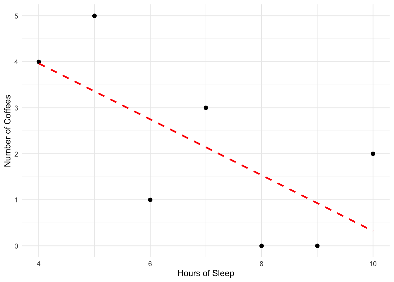
These points show a general trend down and to the right. That is, on days where we have a higher-than-average value for Hours of Sleep, we see lower-than-average value for Number of Coffees. This tells us that the two variables are negatively related.
When discussing a scatterplot, we typically say that the relationship is either positive or negative, or there is no linear relationship. If there is a relationship, we describe it as strong if the observations follow the pattern almost perfectly, moderate if the observations only show a rough trend, and weak if there is barely a noticeable pattern.
In our dataset for Lori Bilmore, we would say that the relationship between her hours of sleep and her cups of coffee is moderate and negative - which, as we would hope, matches the conclusion we came to by computing the sample correlation!
9.3.1 Linear relationships
What about when variables have no linear relationship; i.e, when the correlation is 0? This might mean that there is no pattern at all in the scatterplot; the points are simply a random cloud with no pattern “up to the right” or “down to the right”.
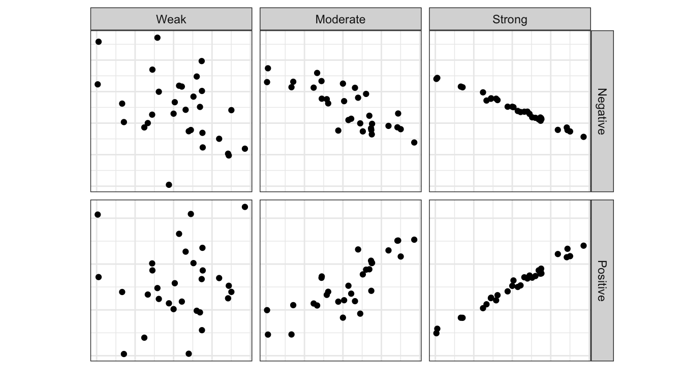
However, remember that correlation measures whether these two variables vary together; i.e., if one is higher than average, does this tell you that the other is probably also higher than average? There are plenty of more complex relationships than a simple higher/lower pattern. For example, the following scatterplots all represent data with correlation of 0:
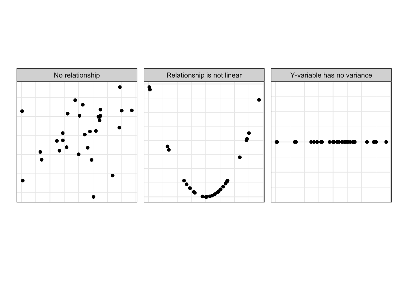
In the first scatterplot, we can see that these variables follow no pattern in the pairs of observed values.
In the second scatterplot, there is a very strong pattern! And it’s true that when the x-variable is higher than average, the y-variable is also higher than average. But it’s also true that when the x-variable is lower than average, the y-variable is higher than average! So, with a trend up to the right and up to the left, is this a positive or negative relationship? It’s neither; this relationship cannot be captured using a linear measurement like correlation.
In the third scatterplot, there is no variability in the observations of the y-variable. If we can’t observe different values, we can’t make any claims about how those values change in relation to the x-variable, so we are forced to conclude no relationship is seen in this data.